Monte Carlo Localisation (MCL) - Part 1: Bayesian Estimation
In this series of posts, I’ll be explaining the Monte Carlo Localisation algorithm, its components and some of its variants through interactive demos. The aim of these posts isn’t to rigorously go through the theory, but rather to build an intuition of how the algorithm works.
This particular post will introduce the localisation problem briefly and how bayesian estimation can be used to solve it.
The Localisation Problem
In order for a robot to know where it is in an environment that lacks a global positioning system (e.g. indoors where GPS is not available), it must rely on its sensors to localise itself. However, most sensors suffer from errors that can build up over time, for example inertial sensors drift over time and encoders can build up errors due to wheel slippage.
Consequently, an effective localisation algorithm must be able to correct for these errors. One way to achieve this is by thinking about the position of the robot probabilisticly rather than deterministically. This means modelling the position of the robot using a probability distribution that reflects the uncertainty introduced by sensing errors.
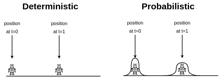
The above figure illustrates the difference between the two ways of thinking about the robot’s position. Deterministically, the robot can only be in one position at any given point in time. As a result, the deterministic estimate would diverge over time. However, when using a probability distribution, we can consider a range of positions and assign different probabilities to positions over this range, based on what we know.
This probability distribution can be updated over time as our belief changes. For example, if we instruct our robot to move at a speed of 1 m/s, but we know that it actually tends to moves 1±0.2 m/s, then we can represent this uncertainty in our belief by spreading it out over a larger range and decreasing our confidence in any particular position as illustrated in the above diagram.
On the other hand, if we have a sensor that can detect where we are in the environment then we can update our probability distribution to increase our confidence in the position detected by the sensor and decrease the spread of the belief. To achieve this, we need a way of updating our belief based on new evidence. Enter Bayesian Estimation!
Bayesian Estimation
I will not go into the detail of how Bayes’ Theorem works here because others have done a much better job at explaining it than I can - I recommend 3Blue1Brown’s video, embedded below. Instead I’ll focus on how the theorem can be used for robot localisation.
Put simply, Bayes’ Theorem, shown below, describes the probability of an event (A) occurring, given our prior knowledge (B) about the event.
\[\begin{equation} p(A|B) = \frac{p(B|A) \cdot p(A)}{p(B)} \label{eq:bayes} \end{equation}\]The same theorem can also be used to express the probability of an event (A) occurring, given multiple other events (B and C):
\[\begin{equation} p(A|B,C) = \frac{p(B|A,C) \cdot p(A|C)}{p(B|C)} \label{eq:bayes_conditioned} \end{equation}\]In the context of robot localisation events A, B and C can be defined as:
- A: The position of the robot at time $t$, denoted as $x_t$.
- B: A series of sensor readings observed by the robot up to time $t$, denoted as $z_{1:t}$.
- C: A series of actions taken by the robot up to time $t$, denoted as $u_{1:t}$.
See appendix at the end of the page for the derivation of the above equation.
In other words, this is the probability that the robot is at position $x$ at time $t$ given all the actions it took and all the observations it made up to time $t$. This is known as the robot’s belief about $x$ at time $t$, which can also be denoted as $bel(x_t)$. This relationship is really powerful because it provides us with a way of estimating the robot’s belief (i.e. where it thinks it is), based on its actions (i.e. how it moved) and what it observed through its sensors.
Note that we can express the denominator of equation $\eqref{eq:bayes_localisation}$ as a normalisation factor:
\[\begin{equation} bel(x_t) = \eta \cdot p(z_t|x_t,z_{1:t-1},u_{1:t}) \cdot p(x_t|z_{1:t-1},u_{1:t}) \label{eq:bayes_localisation_normal} \end{equation}\]See appendix at the end of the page for a more detailed explanation of this.
Ideally we want to update this belief iteratively: as the robot moves and obtains new sensor readings, it updates its belief. However, the formula in its current form doesn’t really allow us to do that, so we will have to simplify it using some assumptions and probability laws, in order to reach an iterative algorithm. In the next two sections, I will present this iterative algorithm, known as Bayes Filter, first then go through its derivation.
Bayes Filter
\begin{algorithm}
\caption{Bayes Filter}
\begin{algorithmic}
\Function{BayesFilter}{$bel(x_{t-1}), u_t, z_t$}
    \FOR{all $x_t$}
        \STATE $\overline{bel}(x_t) = \int p(x_t|u_t,x_{t-1}) bel(x_{t-1}) dx_{t-1}$
        \STATE $bel(x_t) = \eta \cdot p(z_t|x_t) \overline{bel}(x_t)$
    \ENDFOR
    \RETURN $bel(x_t)$
\EndFunction
\end{algorithmic}
\end{algorithm}
The algorithm presented above takes in the belief at the previous time step, $bel(t-1)$, the action taken by the robot at the current time step, $u_t$, and the sensor measurement observed by the robot at the current time step, $z_t$. The algorithm then performs two key steps:
- Prediction: this step is performed on line 3 and it predicts where the robot is, purely based on its motion. For example, if the robot has moved 1 metre to the right, then the belief is shifted by 1 metre to the right and the spread of the belief increases based on the modelled uncertainty.
- Measurement Update: this step is performed on line 4 and it “corrects” the prediction made in the previous step, by incorporating the sensor measurement observed by the robot. This has the effect of increasing the confidence in the belief and decreasing the spread.
To get a better feel of how this algorithm works, try the interactive demo below. In this demo, we have a robot that operates in a 1 dimensional world. The robot can move left or right by 1 metre at a time; however, due to errors in its encoders it can’t be 100% certain about its position. The plot below the robot represents $bel(x_t)$ across all $x$; in other words, the higher the bar at a given position the more likely that the robot believes that it is in this position. At the start of the demo (or after pressing “Reset Probabilities”), all the bars are of an equal height, which indicates that the robot believes that it is equally likely to be in any of the positions.
Every time you press “Move left” or “Move right”, the robot executes the prediction step of the Bayes Filter. In other words, it updates its belief purely based on its motion.
The robot also has a sensor that can detect doors. If you tick the “Enable sensor?” checkbox then as the robot moves, it will also execute the measurement update step, thus correcting the estimate obtained by the prediction step based on the sensor measurement observed by the robot. Notice how the confidence and spread of the belief change when the sensor is on and the robot detects a door.
Try turning the sensor on and moving the robot to the position where the door is, you’ll notice that the robot becomes quite certain about where it is. Now turn off the sensor and try moving the robot. Notice how the belief starts to spread, due to the modelled uncertainty in this motion.
The above demo was inspired by a great lecture on youtube.
Bayes Filter Derivation
Starting from equation $\eqref{eq:bayes_localisation_normal}$ The first assumption we will make is that if the robot’s current state is known then we don’t need to know its previous states in order to be able to estimate its future states. For example, if we know where the robot is at this point in time, what action it took and what sensor observation it made then we can estimate where it is going to end up next without knowing where it was before.
Formally, this is known as the Markov assumption. Strictly speaking, we can’t really fully define the current state of the robot. For that we would have to know precisely where the robot is, where every obstacle (including unmodelled obstacles such as a passing human) is and many other things, which is not practical. However, in practice, probablistic algorithms are quite robust to these discrepancies.
Articulating this assumption into maths, we can simplify $p(z_t|x_t,z_{1:t-1},u_{1:t})$ into $p(z_t|x_t)$, because we assume that what the robot is currently observing, $z_t$, is only affected by its current position, $x_t$:
\[\begin{equation} bel(x_t) = \eta \cdot p(z_t|x_t) \cdot p(x_t|z_{1:t-1},u_{1:t}) \end{equation}\]We will denote $p(x_t|z_{1:t-1},u_{1:t})$ as $\overline{bel}(x_t)$, thus arriving at the measurement update step of the algorithm:
\[\begin{equation} bel(x_t) = \eta \cdot p(z_t|x_t) \cdot \overline{bel}(x_t) \label{eq:bayes_markov} \end{equation}\]Using the law of total probability we can expand $\overline{bel}(x_t)$:
\[\begin{equation} \overline{bel}(x_t) = p(x_t|z_{1:t-1},u_{1:t}) = \int p(x_t|x_{t-1},z_{1:t-1},u_{1:t}) \cdot p(x_{t-1}|z_{1:t-1},u_{1:t}) dx_{t-1} \end{equation}\]Relying on the Markov assumption again, we can simplify $p(x_t|x_{t-1},z_{1:t-1},u_{1:t})$ into $p(x_t|x_{t-1},u_t)$, since past measurements, $z_{1:t-1}$, and actions, $u_{1:t-1}$ are not needed if $x_{t-1}$ is known. We can also remove $u_t$ from $p(x_{t-1}|z_{1:t-1},u_{1:t})$, since $x_{t-1}$ is only dependent on the actions up to time $t-1$:
\[\begin{equation} \overline{bel}(x_t) = p(x_t|z_{1:t-1},u_{1:t}) = \int p(x_t|x_{t-1},u_t) \cdot p(x_{t-1}|z_{1:t-1},u_{1:t-1}) dx_{t-1} \label{eq:belbar} \end{equation}\]Notice that $p(x_{t-1}|z_{1:t-1},u_{1:t-1})$ is equivalent to $bel(x_{t-1})$, so we can rewrite $\eqref{eq:belbar}$ as:
\[\begin{equation} \overline{bel}(x_t) = p(x_t|z_{1:t-1},u_{1:t}) = \int p(x_t|x_{t-1},u_t) \cdot bel(x_{t-1}) dx_{t-1} \end{equation}\]This equation is the same as the prediction step of the algorithm.
Implementing the algorithm
Now that we have arrived at a probabilistic localisation algorithm, it would be nice to implement it on a real robot! However, to be able to do that we need to do 3 things:
- Calculate $p(x_t|x_{t-1},u_t)$ to be able to work out the prediction step. In order to do this, we need to come up with a motion model that estimates the probability of ending up at position $x_t$ given our starting position, $x_{t-1}$ and the action (motion) we took, $u_t$.
- Calculate $p(z_t|x_t)$ to be able to work out the measurement update step. In order to do this, we need to come up with a measurement model that estimates the probability of observing the current measurement, $z_t$, given our current position $x_t$.
- The algorithm presented here is a continuous algorithm, it integrates over the continuous space of $x$; however, in order to implement it on a digital computer, we must come up with a way of discretising the space of $x$.
In the next 3 articles, I will be covering each of these topics in turn.
References and Resources
- Probabilistic Robotics. This is a fantastic book to learn more about about the word of probabilistic robotics.
Appendix
Derivation of equation $\eqref{eq:bayes_localisation}$
Let’s start from equation $\eqref{eq:bayes_conditioned}$ and substitute A, B and C for $x_t$, $z_{1:t}$ and $u_{1:t}$ respectively:
\[\begin{equation} p(x_t|z_{1:t},u_{1:t}) = \frac{p(z_{1:t}|x_t,u_{1:t}) \cdot p(x_t|u_{1:t})}{p(z_{1:t}|u_{1:t})} \label{eq:bayes_localisation_1} \end{equation}\]$z_{1:t}$ is a series of data points $(z_1, z_2, …, z_{t-1}, z_t)$, so we can rewrite it as $(z_{1:t-1}, z_t)$. Substituting this broken down version of $z_{1:t}$ into equation $\eqref{eq:bayes_localisation_1}$, we get $p(x_t|z_t, z_{1:t-1}, u_{1:t})$. To expand this, we can refer back to $\eqref{eq:bayes_conditioned}$, but this time we substitute A, B and C for $x_t$, $z_{1:t}$ and $z_{t-1}, u_{1:t}$ respectively, thus reaching equation $\eqref{eq:bayes_localisation}$:
\[p(x_t|z_t,z_{1:t-1},u_{1:t}) = \frac{p(z_t|x_t,z_{1:t-1},u_{1:t}) \cdot p(x_t|z_{1:t-1},u_{1:t})}{p(z_t|z_{1:t-1}, u_{1:t})}\]The normalisation factor in Bayes’ theorem
An alternative way of thinking about Bayes’ theorem is in terms of likelihood, rather than probability:
\[\begin{equation} P(A|B) \propto P(B|A) \cdot P(A) \end{equation}\]This means that the likelihood of a hypothesis (A) being true given the evidence (B) is proportional to the product of:
- The probability of the evidence being observed given the hypothesis is true, $p(B|A)$.
- The probability of the hypothesis being true.
In order to obtain a probability distribution from the above relationship, the sum of over all possible hypotheses (A) must be 1. We can multiply a normalisation factor, $\eta$, by $P(B|A) \cdot P(A)$ for each hypothesis (A):
\[\begin{equation} P(A|B) = \eta \cdot P(B|A) \cdot P(A) \end{equation}\]This normalisation factor is give by:
\[\begin{equation} \eta = \int P(B|A) \cdot P(A) dA = p(B) \end{equation}\]